Area-under-curve (AUC) in PET

Most analysis methods of PET data require calculation of integral over time ("area-under-curve") of the input function, for instance in FUR and Patlak plot; in other cases, including compartmental models the integration of plasma or blood curve is less obvious but still done by the analysis tools. Integration of dynamic PET data is needed in Logan plot, SUV, and SUVR calculations. In addition, AUC from time zero to infinity needs to be estimated in dosimetry and pharmacokinetics.

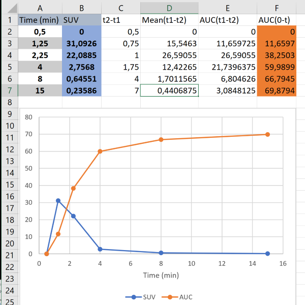
The AUC of plasma and blood time-activity curves (PTAC and BTAC, respectively) can be calculated by dot-to-dot integration ("trapezoidal rule"), when separate blood samples have been collected manually; each curve value then represents the radioactivity concentration at the time when blood sample was withdrawn (Fig. 1):

AUC calculation in spreadsheet — **Figure 1. AUC calculation:** Blood samples are collected at discrete time points (column A) and sample radioactivity concentrations are listed in SUV units (column B). Concentration curve is plotted in blue. AUC is calculated stepwise between each sample time (column E), by multiplying the sample time difference (column C) and the mean of sample concentrations (column D). AUCs are then summed (column F). The sum of AUC from time zero to each sample point is plotted in orange colour. The unit of AUC is (time unit)×(concentration unit).

Analysis software calculates the integrals similarly. Integrals can also be computed using command-line program interpol with option -i.

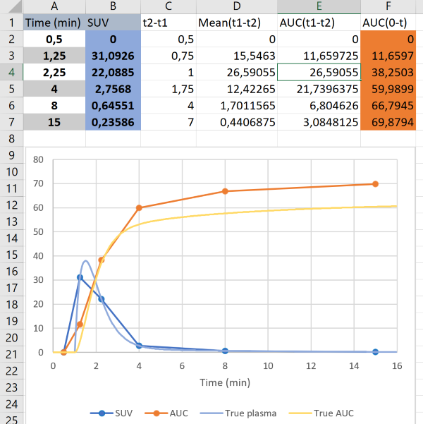
Since the blood samples in this example are withdrawn relatively infrequently, errors will be introduced if the measured curve does not well represent the true kinetics of the input function. Below, the true input concentration curve and AUC are plotted with the same data as in the previous figure, to show that large error in AUC may result from too sparse blood sampling (Fig. 2):

**Figure 2. Effect of sparse sampling on AUC calculation:** Light blue curve represents the true plasma curve, and yellow line represents the true AUC. Since the sampling is too sparse, the true shape of the plasma curve was missed, in this example leading to overestimation of AUC between the two first samples, underestimation of AUC between the next samples, and again overestimation between the 3rd and 4th samples. By definition, also the errors are summed in AUC calculation, leading to overestimated (in this example) AUC for the whole time time range.

Therefore, it is important that blood sampling is frequent enough when the concentration is rapidly changing. In bolus infusion PET studies, the plasma/blood peak region is the most crucial part (Fig. 3):

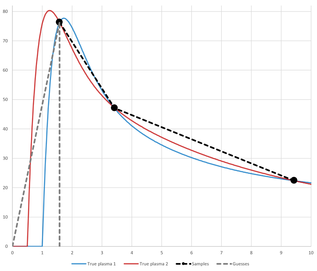
**Figure 3. Effect of missing the TAC peak:** In this example the black circles represent the measured plasma concentrations. True plasma TAC could be either the blue or red curve. Since the blood sampling has missed the part where concentration is still zero or increasing, we have no means to guess whether the curve peak was before or after the first measured sample. The initial part of AUC must be estimated using either of the methods depicted with the grey dashed lines. Both methods will lead to error, and the magnitude and direction of the error is unknown and dependent on the true plasma curve.

With the command-line program interpol user can optionally select the method how to estimate the initial AUC. Program inpstart can be used in scripts to roughly check that the peak of input curve was not missed, but it must not be used to replace visual verification of the data quality.

One solution is to measure blood TAC using automatic blood sampling system (ABSS), although it has its own problems. In theory, fitting a mathematical function to the sparse input data may help in integration and interpolation; but since the measured data is noisy, and functions are only empirical representations of typical tracer kinetics after successful tracer administration, fitting would just increase uncertainty in the analysis process.

In pharmacokinetic studies and and in measurement of GFR, blood sampling usually starts few minutes after the bolus injection, but calculation of clearance requires that AUC_0-∞ is measured. The initial part has often been estimated with back-extrapolation, which may lead to "mixing" or "bolus" error.

AUC from time frame data

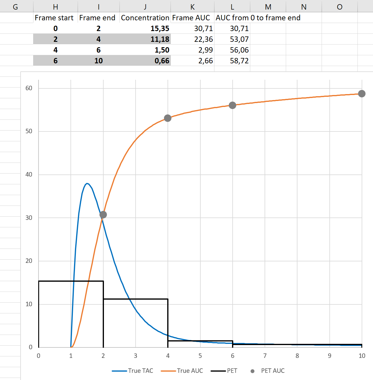
Tissue time-activity curves (TTACs) and image derived input curves, based on PET measurements, and blood time-activity curves (BTACs) collected using ABSS are collected as mean concentrations during specified time frames. The events (counts) have to be collected over the certain time "frame" to achieve acceptable count statistics, and the number of measured events are then divided by the time frame length to obtain the count rates (counts/s), which are further calibrated to radioactivity concentrations (Bq/mL) based on the measured volume and calibration coefficients. If time frames are sufficiently short, we can assume that the average tracer concentration during the time frame represents the instantaneous concentration at frame middle time point ("midframe approximation", see Buchert et al., 2003). If concentration changes markedly during the time frame, then the midframe approximation is not valid (Figs 4a and 4b).

To obtain AUC during the time frame, the radioactivity concentration can be simply multiplied by the frame length, and the AUC obtained this way is not biased at the frame end times even with long the frame lengths (Figs 4a and 4b), except for the small error introduced by decay correction which assumes that concentration does not change during the frame. If integral needs to be assessed between the frame start and end times, then some assumptions must be made about the concentration changes during the time frame.

AUC from PET data with time frames — **Figure 4a. AUC from time frame data:** Blue line represents the true time-activity curve, and orange line its AUC from time zero. Black bars represent the PET frames. For each time frame, AUC (column K) can be calculated as concentration average during the frame (column J) multiplied by frame duration (column I minus column H). AUC from time zero to the end of PET frame (column L, grey circles) can be calculated as sum of AUCs for individual frames.

AUC from PET data with long frames — **Figure 4b. AUC from time frame data:** In this example the same data is used as in previous figure, except that frame lengths are now longer. As can be seen, AUC can still be calculated correctly, but TAC shape is very poorly represented by the frame averages.

The fact that AUC can be correctly calculated from PET data with long frames can be utilized in PET scan protocols for Patlak and Logan plots; only AUC is needed from the early time range for these graphical analysis methods, and therefore the first image time frames can be long.

Analysis software calculates the integrals based on image time frames, and also regional TTACs may preserve frame start and end times. Integrals, considering the frames lengths, can also be computed using command-line programs dftinteg and imginteg.

AUC from zero to infinity

The AUC from 0 to infinite time, AUC_0-∞, is needed in calculation of dosimetry and plasma pharmacokinetics for PET radioligands. For the sampling duration the AUC can be determined by the trapezoidal rule, but since the last measured concentration is not zero, stopping AUC calculation at that time point would underestimate the AUC_0-∞. Therefore, the rest of the curve must be extrapolated with exponential function. In practise, line is fitted to the plot of the natural logarithm of tracer concentration against time. This can be done e.g. using program paucinf, or with Excel (Zhang et al., 2010). The slope of the linear part of the plot, A, is negative and equals -k_el; the slope and the y axis intercept of the fitted line (B) can be used to calculate the integral from the last sample time (t_LS) to infinity:

${AUC}_{t_{LS}-\infty} = \frac{{e^B} * e^{(A*t_{LS})}}{-A}$

, which is then added to the AUC calculated from the sampled time range.

Example

Example dosimetry data, stored in PMOD-formatted text file kanit.tac:

time[hour]	kani1	kani2
0,002	1,843998941	12,48854572
0,006	26,57880893	27,15690636
0,010	27,81422174	27,2508763
0,015	24,95289268	30,11531703
0,021	24,6088121	27,46352825
0,029	23,94164827	26,56452008
0,038	26,05074671	28,27240406
0,046	27,18322752	24,62507584
0,058	26,82812168	27,74892528
0,075	24,13405129	30,03561905
0,125	23,84561008	25,51318302
0,208	23,35385837	26,92998525
0,292	22,64704041	26,42876143
0,375	22,64042787	26,72444256
0,458	22,88441149	25,14929462
0,542	22,99261657	25,82539875
0,625	22,94944039	25,73525504
0,750	21,53232992	25,28724687
0,917	20,87775579	25,03024888
24,000	14,519465	17,0535419
48,000	14,52988259	12,33580858
144,000	5,167555956	4,510780064
216,000	3,432414852	2,703595935
288,000	1,335165334	1,105938208
360,000	0,649894738	0,500921454
432,000	0,31633773	0,226886368
504,000	0,153978104	0,102765461
576,000	0,074949189	0,046546384
648,000	0,036481687	0,021082626
720,000	0,017757543	0,009549123
792,000	0,008643524	0,004325161
864,000	0,004207255	0,00195903
936,000	0,002047891	0,000887319
984,000	0,001267201	0,000523326
1056,00	0,000616813	0,000237034

is analyzed with paucinf, saving results in HTML table format for easy importing into Excel (Fig. 5a), and plotting the line fits with ln-transformed data (Fig. 5b):

paucinf -svg=kanit.svg kanit.tac kanit.html

If you are allergic to command line, you can write the above command in to text file, and save it with extension .bat (in Windows), and then double-click the .bat file icon.

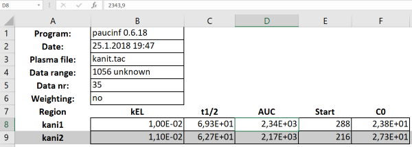
AUC results computed using paucinf — **Figure 5a.** AUC from time zero to infinity estimated using `paucinf`, saved in HTML table format, and drag-and-dropped into Excel. "Start"-column gives the sample time from which the linear fit was started.

Line fits using paucinf — **Figure 5b.** Line fits to the ln-transformed data, as saved in SVG format. Depending on the kinetics and concentration units, ln-transformed data can be negative, when measured values are <1.0; this does not affect the calculation, but measured values ≤0.0 would lead to an error.

By default, paucinf determines automatically the best time range for the linear fitting. The time range can be optionally refined.

This approach only works with curves approaching zero, which is the case in dosimetry calculations, because the activity data is not corrected for physical decay. In pharmacokinetic calculations decay corrected activity concentrations are used; although concentrations eventually would approach zero, during the time scope of PET scans the concentrations often reach an apparently steady level well above zero; extrapolation with line fitting to ln-transformed curves does not work in that case, but at least two-exponential function is required, and extrapolation and especially AUC calculation will be prone to large errors.

Literature

Buchert R, van den Hoff J, Mester J. Accurate determination of metabolic rates from dynamic positron emission tomography data with very-low temporal resolution. J Comput Assist Tomography 2003; 27(4): 597-605. doi: 10.1097/00004728-200307000-00026.

Häggström I, Axelsson J, Schmidtlein CR, Karlsson M, Garpebring A, Johansson L, Sörensen J, Larson A. A Monte Carlo study of the dependence of early frame sampling on uncertainty and bias in pharmacokinetic parameters from dynamic PET. J Nucl Med Technol. 2015; 43: 53-60. doi: 10.2967/jnmt.114.141754.

Chen K, Huang S-C, Feng D. New estimation methods that directly use the time accumulated counts in the input function in quantitative dynamic PET studies. Phys Med Biol. 1994; 39: 2073-2090. doi: 10.1088/0031-9155/39/11/017.

Kolthammer JA, Muzic RF. Optimized dynamic framing for PET-based myocardial blood flow estimation. Phys Med Biol. 2013; 58: 5783-5801. doi: 10.1088/0031-9155/58/16/5783.

Li X, Feng D. Towards the reduction of dynamic image data in positron emission tomography studies. Comput Meth Progr Biomed. 1997; 53: 71-80. doi: 10.1016/S0169-2607(97)01812-9.

Mazoyer BM, Huesman RH, Budinger TF, Knittel BL. Dynamic PET data analysis. J Comput Assist Tomogr. 1986; 10(4): 645-653. doi: 10.1097/00004728-198607000-00020.

Wallstén E, Axelsson J, Karlsson M, Riklund K, Larsson A. A study of dynamic PET frame-binning on the reference Logan binding potential. IEEE TRPMS 2017; 1(2): 128-135. doi: 10.1109/TNS.2016.2639560.

Zhang Y, Huo M, Zhou J, Xie S. PKSolver: An add-in program for pharmacokinetic and pharmacodynamic data analysis in Microsoft Excel. Comput Methods Programs Biomed. 2010; 99: 306-314. doi: 10.1016/j.cmpb.2010.01.007.

Tags: AUC, TTAC, PTAC, Time frame, FUR, Simulation, Extrapolation

Updated at: 2019-02-13
Created at: 2018-01-23
Written by: Vesa Oikonen

Area-under-curve (AUC) in PET

AUC from time frame data

AUC from zero to infinity

Example

See also:

Literature