MPI with chemical microspheres

Labelled small microspheres that are trapped in tissue capillaries can be used to quantify nutritive blood flow to tissue (perfusion). Similarly, perfusion could be assessed with labelled radiopharmaceutical that is rapidly and irreversibly taken up by cells.

Concentration of the tracer in the blood (C_B) is an average of concentrations in plasma (C_P) and red blood cells (C_RBC), weighted by haematocrit (HCT):

$C_{B}(t) = (1 - {HCT}) \ C_{P}(t) + {HCT} \ C_{RBC}(t)$

The arterial plasma TAC, not the whole blood TAC, is the correct input function in this model since the radiopharmaceutical in blood cells is assumed to be trapped. Since we want to assess blood flow instead of plasma flow, we write the differential equations for tissue and blood cell concentrations as

$\frac{dC_{T}(t)}{dt} = K_1 \ (1 - {HCT}) C_{P}(t)$ $\frac{dC_{RBC}(t)}{dt} = {k_C} \ (1 - {HCT}) C_{P}(t)$

, where (1-HCT)×C_P is the plasma radioactivity per volume of blood. After integration and rearrangement,

$\frac{C_{T}(T)}{K_1} = \frac{C_{RBC}(T)}{k_c} = \int\limits_{0}^{T} (1 - {HCT}) C_{P}(t) dt$

, which clearly shows that in this chemical microsphere model the TACs of muscle tissues and RBCs have the same shape, the integral of plasma TAC as a function of time, but with their own scaling factors.

Solving Eq 4 for C_RBC(t) and substituting it into Eq 1 gives equation

$C_{B}(t) = (1 - {HCT}) \ C_{P}(t) + \frac{k_c {HCT}}{K_1} \ C_{T}(t) \nonumber$

which can be solved for (1-V_B)×C_P(t), which is then substituted in Eq 2, giving

$\frac{dC_{T}(t)}{dt} = K_1 \ C_{B}(t) - k_c \ {HCT} \ C_{T}(t)$

This is similar to the differential equation of the commonly used reversible one-tissue compartment model with k₂=k_C×HCT.

$\frac{dC_{T}(t)}{dt} = K_1 \ C_{B}(t) - k_2 \ C_{T}(t)$

Practical compartmental model for MPI with chemical microspheres — **Figure 2.** Practical compartmental model for myocardial perfusion imaging using PET and chemical microspheres, when arterial plasma TAC is not available, as assumed in Fig 1, but blood TAC can be measured from ROI placed in the LV cavity of the heart. Model mimics the commonly used reversible two-compartment model (one-tissue compartment model); when applied to the case of chemical microspheres (trapping in cells), the interpretation of the k₂ parameter is different: k₂ is the product of haematocrit and the rate constant of tracer trapping in blood cells, k_C × HCT.

The regional TACs from myocardial PET studies are distorted by Spillover and partial volume effects. In theory, this can be accounted for by modelling the left ventricular (LV) muscle and cavity TACs as:

$C_{PET}(t) = \alpha \times C_{T}(t) + V_{B} \times C_{B}(t) \nonumber$ $C_{CAV}(t) = \beta \times C_{B}(t) + (1 - \beta) \times C_{T}(t) \nonumber$

, where α is the tissue fraction inside myocardial muscle ROI and V_B is the blood volume fraction, and β is the recovery coefficient of LV cavity ROI. The V_B is assumed to represent the spillover and partial volume effects from the blood in LV cavity; the contribution of vascular blood volume in muscle is assumed to be negligible; majority of that would be venous blood, with curve shape determined by the concentration in red blood cells and thus similar to the muscle tissue in this model (see Eq 4).

The β is dependent on the image resolution, and could be measured with [¹⁵O]CO PET. In myocardial radiowater PET studies the model can be first fitted to the data from a large ROI covering most of the left ventricular myocardium (possibly excluding septum and areas with marked spillover from the liver), enabling calculation of C_B(t), which is then used for analysis of smaller myocardial regions (Iida et al., 1988, 1991, and 1992). The resolution of modern PET may allow using the blood curve derived from a tiny ROI placed in the LV cavity directly, and therefore we assume that β=1, and

$C_{B}(t) = C_{CAV}(t) \nonumber$

While the α can be estimated in myocardial PET studies with radiowater that is a diffusible tracer with known equilibrium tissue distribution volume, that is not possible with a trapped radiopharmaceutical. Instead we must draw muscle ROI avoiding carefully the tissues outside of the heart, and use the simple geometrical model

$C_{PET}(t) = (1 - V_{B}) C_{T}(t) + V_{B} C_{B}(t)$

C_T(t) and dC_T(t)/dt are solved from this equation and its derivative, respectively, and placed in Eq 6, providing the ODE and its integral

$\frac{dC_{PET}(t)}{dt} = V_{B} \frac{dC_{B}(t)}{dt} + \left[ (1-V_{B})K_1 + V_B k_2 \right] \ C_{B}(t) \ - k_2 \ C_{PET}(t)$ $C_{PET}(T) = V_{B} C_{B}(T) + \left[ (1-V_{B})K_1 + V_B k_2 \right] \int\limits_{0}^{T} C_{B}(t)dt \ - k_2 \int\limits_{0}^{T} C_{PET}(t)dt$

This multilinear equation has three parameters, V_B, K₁, and k₂=k_C×HCT, and all concentrations are measured with PET. The parameters can be fitted with non-linear optimisation methods, or solved using non-negative least squares (NNLS) optimisation method, like has been done for example to fit muscle data from radiowater PET studies (Burchert et al., 1997). The NNLS method is computationally very fast, allowing pixel-by-pixel calculation and production of parametric K₁ and V_B image.

The last of the parameters, k₂=k_C×HCT, is related only to the kinetics of tracer in blood and plasma, and therefore common to all tissue regions. Therefore it is possible to either perform the fits of all tissue regions simultaneously, with a single k₂ parameter, or to first fit a large (less noisy) myocardial region, and fit the (noisier) TACs of smaller myocardial regions with fixed k₂. If k₂ is known, the remaining two parameters can be solved using NNLS from multilinear equation

$C_{PET}(T) + k_2 \int\limits_{0}^{T} C_{PET}(t)dt = \ V_{B} \ \left( C_{B}(T) + k_2 \int\limits_{0}^{T} C_{B}(t)dt \right) \ + (1-V_{B})K_1 \ \int\limits_{0}^{T} C_{B}(t)dt$

With k₂, the plasma component of measured, discrete blood data curve could be computed from ODE that could, for example, be solved using implicit second-order Adams-Moulton corrector, resulting in equation

$(1 - HCT) \ C_{P}(T) = \frac{ C_{B}(T) - k_2 \ \left[ \int\limits_{0}^{T-\Delta t} (1 - HCT) C_{P}(t)dt + \ \frac{\Delta t}{2} (1 - HCT) C_{P} (T - \Delta t) \right] }{1 + \frac{\Delta t}{2} k_2}$

, where Δt is the sample time difference. Program b2ptrap can make the plasma curve with this method using known k₂, or it can fit the k₂ based on blood data alone with assumption that radioactivity in plasma is zero after a certain time. Program fitmtrap, which can be used to fit the model in Eq 10 to regional data, can also make the plasma curve with this method.

If both arterial plasma and blood curves would available, a very simple linear equation can be formed with only two parameters to be fitted:

$C_{PET}(T) = V_{B} \ C_B(t) + (1-V_{B})K_1 \ \int\limits_{0}^{T} (1 - {HCT}) \ C_{P}(t) dt$

The reversible one-tissue model with parameters V_B, K₁, and k₂ is included in all PET modelling software, and the parameters V_B and K₁ from those tools can directly be interpreted as the parameters of the chemical microsphere model.

K₁ and perfusion

The unidirectional transport rate of the radioligand from the blood to the tissue (K₁) and blood flow (F), according to the Fick's principle and Renkin-Crone capillary model, are related by first-pass extraction fraction E,

$K_1 = F \times E \nonumber$

, where E depends on perfusion, and the product of capillary permeability P and capillary surface area S, PS. Only highly diffusive (E ≅ 1) tracers can be used to reliably measure regional perfusion. If E is substantially reduced when perfusion is high, a non-linear function is needed to convert K₁ to perfusion. E cannot be determined from PET data, but comparison of K₁ estimates to perfusion values measured with gold-standard methods can provide the non-linear function that can be used to obtain perfusion from K₁.

Simulations

Late-time tissue-to-blood ratio (TBR)

An intravenously administered radiotracer that traps into cells is rapidly cleared from the plasma. As plasma curve approaches zero, its area-under-curve (integral) stabilizes to a certain level. Likewise, the concentrations in blood cells and tissue stabilize to a level determined by the integral (area-under-curve) of the plasma concentration and the rate constants k₂=k_c×HCT and K₁ (see Eq 4). At this phase, since C_P=0, the concentration in blood is

$C_B = {HCT} \ C_{RBC} \nonumber$

and the late-time regional tissue-to-blood ratio, based on Eq 7 and C_T/C_RBC from Eq 4, is

$\frac{C_{PET}}{C_B} = V_B + \frac{(1 - V_B) \ K_1}{k_C \ {HCT}}$

We can see that the late-time TBR correlates with K₁, but is affected by V_B (which represents the partial volume and spillover effects in myocardial model) and k₂=k_c×HCT (the rate of tracer uptake in blood cells). The relationship of K₁ and late-time TBR is shown in Fig 3. When K₁ < k_C×HCT, the late-time concentration in myocardial regions will be lower than concentration in blood (LV cavity), which complicates the drawing of regions-of-interest to areas with perfusion defect.

Haematocrit has a linear effect on late-time TBR (Eq 13). The tissue uptake is related to plasma flow, and its proportion of blood flow, (1-HCT)×F, is higher when haematocrit is lower, which explains the higher late-time TBR with lower haematocrit in the right panel of Fig 3.

The late-time TBR correlates linearly with K₁ when other model parameters are assumed constant. V_B however has strong effect on the regional tissue concentrations. When drawing the regions on the PET image it is difficult to control the contribution of blood in LV cavity to the muscle regions; usage of tissue-to-blood ratio (TBR) or late-time SUV in quantification of myocardial perfusion cannot therefore be recommended, especially as the compartment model solutions are readily available, providing K₁ that is not affected by V_B, k_C, or haematocrit. However, the late SUV or TBR image may be useful in visual analyses.

Correlation of late-time TBR and K1 — **Figure 3.** The relationship between late-time TBR (C_PET/C_B) and K₁ (range 0.0-5.0 or 0.0-1.0) as calculated from Eq 13. When K₁ decreases towards zero, late-time TBR approaches the V_B. *Left:* Constant k_C=0.6 and HCT=0.39, with different V_B values. *Middle:* Same data but limited to lower K₁ range. *Right:* Constant V_B=0.25 and k_C=0.6, with different haematocrit (HCT).

Correlation of late-time TBR and K1 when K1 is less than one — **Figure 3.** The relationship between late-time TBR (C_PET/C_B) and K₁ (range 0.0-5.0 or 0.0-1.0) as calculated from Eq 13. When K₁ decreases towards zero, late-time TBR approaches the V_B. *Left:* Constant k_C=0.6 and HCT=0.39, with different V_B values. *Middle:* Same data but limited to lower K₁ range. *Right:* Constant V_B=0.25 and k_C=0.6, with different haematocrit (HCT).

Kinetic data simulation

In this simulation, a sum of exponentials function (Feng et al., 1993a and 1993b) is used to describe the input function of the model, the arterial plasma curve (C_P(t)), shown in Fig 4. In the present model the intravenously administered radiotracer is assumed to become rapidly trapped in cells, including blood cells, and therefore the function is set to approach zero in few minutes. The tracer concentration in blood cells is simulated based on Eq 3, and the arterial blood curve is calculated as the sum of tracer concentrations in blood cells and plasma (Fig 4).

Blood curve and its components — **Figure 4.** The simulations are based on the arterial plasma curve (C_P) shown in the picture at the middle. Based on that, the concentration in blood cells (C_RBC) is calculated from Eq 3, with HCT=0.39 and k_C=0.60. The picture on the left shows the simulated blood curve (C_B) and its components, (1-HCT)×C_P and HCT×C_RBC. The picture at the middle shows what measured arterial blood and plasma curves would look like, and the plasma-to-blood ratio as function of time is shown in the picture on the right.

Arterial plasma and blood curves — **Figure 4.** The simulations are based on the arterial plasma curve (C_P) shown in the picture at the middle. Based on that, the concentration in blood cells (C_RBC) is calculated from Eq 3, with HCT=0.39 and k_C=0.60. The picture on the left shows the simulated blood curve (C_B) and its components, (1-HCT)×C_P and HCT×C_RBC. The picture at the middle shows what measured arterial blood and plasma curves would look like, and the plasma-to-blood ratio as function of time is shown in the picture on the right.

Myocardial muscle tissue curves (C_T) were then simulated using Eq 2 with K₁ values ranging from 0.2 to 3.0 mL Blood/(min × mL tissue). These, and previously simulated blood curve, were used to calculate regional muscle curves (C_PET) with different values for V_B (Fig 5).

Simulated regional TACs — **Figure 5.** *Left:* Regional TACs simulated with a range of K₁ values and V_B=0.25. *Right:* Regional TACs simulated with a range (0.1-0.4) of V_B values and K₁=0.8.

Effect of Vb on regional TACs — **Figure 5.** *Left:* Regional TACs simulated with a range of K₁ values and V_B=0.25. *Right:* Regional TACs simulated with a range (0.1-0.4) of V_B values and K₁=0.8.

The simulated TACs reach a steady level ∼5 min after tracer administration, but the exact time depends on the input function and model parameters. As expected, the simulated, noiseless, regional tissue data could be well fitted with reversible one-tissue compartment model using blood curve as input function, and it provided K₁ and V_B estimates that were close to the ones used to simulate the data (results not shown). Extending the PET scan long after the steady phase is achieved would not help the parameter estimation; in real-world PET studies it may be detrimental, if radioactive metabolites of the tracer are released from cells at later times, invalidating the model.

PET image simulation

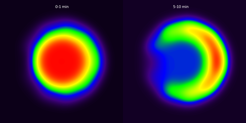
As a rudimentary mock-up of a myocardial dynamic PET image was made by filling segments of a ring with myocardial muscle TACs simulated with different K₁ values, and centre with blood TAC, representing LV cavity (Fig 6 and Fig 7). The input curves simulated previously were used.

K1 values inside simulated image — **Figure 6.** K₁ values inside the simulated image. The segments of the ring represent LV myocardial muscle regions. The centre represents the LV cavity, filled with blood and therefore K₁=0. The image area surrounding the ring is simulated with K₁=0.03 and V_B=0.01. Muscle TACs are simulated with V_B=0.0, since strong Gaussian smoothing is used to simulate partial volume and spillover effects.

Dynamic image was then constructed with these TACs. In this simulation, no noise was added. Partial volume and spillover effects were simulated by strong smoothing with Gaussian filter; Fig 7 shows the sum images from time range 0-1 min and 5-10 min.

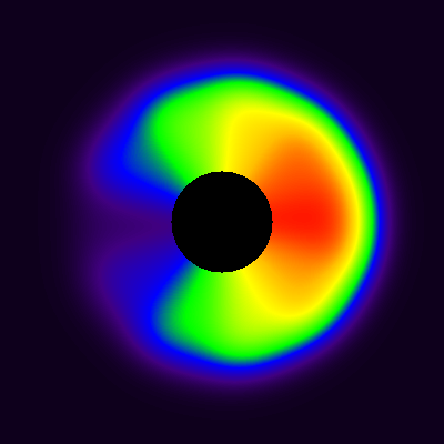
The blood curve from then extracted from middle of the area representing cavity, and model in Eq 9 was applied pixel-by-pixel to the dynamic image, producing parametric V_B and K₁ images (Fig 8). The spillover leads to apparent presence of muscle tissue far inside the cavity, in such extent that K₁ can be estimated there, but not in the middle of the cavity where V_B approaches 1, and K₁ can no longer be estimated (represented by the black hole in the middle of the image where K₁ is set to zero). Partial volume effect leads to underestimation of K₁ in the region where the muscle actually is located, but less so at the border of muscle and cavity, because the spillover between cavity and muscle is corrected in the model (with the model parameter V_B).

Vb image estimated from simulated dynamic image — **Figure 8.** Parametric V_B (left) and K₁ (right) images calculated from simulated dynamic image using Eq 9. The colour scale is the same as in Fig 6.

K1 image estimated from simulated dynamic image — **Figure 8.** Parametric V_B (left) and K₁ (right) images calculated from simulated dynamic image using Eq 9. The colour scale is the same as in Fig 6.

Raw parameter 2 image estimated from simulated dynamic image — **Figure 9.** Image of the raw parameter 2, (1-V_B)×K₁, from a constrained fit (Eq 10), where k₂ is fixed to the median of k₂ from those pixels where V_B and K₁ are within reasonable limits in an initial full model fitting (Eq 9). The colour scale is the same as in Fig 6. The muscle regions could possibly be better identified from this image than from the late scan sum image (Fig 7), but to get less biased perfusion estimates the ROIs should still be drawn closer to the cavity than where the hottest regions in this image are seen. Program imgmtrap was used to compute the parametric images.

The effect of spillover on LV cavity

In the present model and previous simulations the assumption is that true arterial blood curve can be extracted from a small ROI drawn in the middle of the LV cavity. In practise, the blood curve may be contaminated by myocardial muscle curve because of spillover and partial volume effects. In this simulation, the cavity curves were simulated with β values 100%, 95%, 90%, and 85%, meaning contamination of 0%, 5%, 10%, and 15% from myocardium, respectively. Since the level of tissue curve is dependent on perfusion, the simulation is performed with three different K₁ values, 0.5, 1.0, and 2.0. The simulated data were then fitted using fitmtrap according to Eq 9. The model fitted the simulated curves perfectly (not shown). The simulated cavity curves and myocardial curve, and the bias induced to the estimated model parameters, are shown in Fig 10. The simulations suggest that tissue-contaminated blood curve leads to overestimation of all model parameters. The bias in both K₁ and V_B is similar to the contamination-% of the cavity curve. While the higher perfusion leads to higher overestimation of cavity curve, this does not influence the bias in estimated K₁ values, which seems to be overestimated by about the same percentage in all perfusion levels. Most of the bias seems to be absorbed by the parameter k₂.

Effect of spillover and partial volume effect on LV cavity curve when K1=0.5 — **Figure 10.** The effect of spillover and partial volume effects on the blood curves extracted from the LV cavity (left side), and the induced bias on estimated model parameter (right side), with three different perfusion levels (K₁ 0.5, 1.0, and 2.0). In this simulation the V_B in myocardial regions is 0.25 and k₂=0.24. The biases in K₁ and V_B estimates are similar, causing the curves to overlap.

Effect on estimated model parameters when K1=0.5 — **Figure 10.** The effect of spillover and partial volume effects on the blood curves extracted from the LV cavity (left side), and the induced bias on estimated model parameter (right side), with three different perfusion levels (K₁ 0.5, 1.0, and 2.0). In this simulation the V_B in myocardial regions is 0.25 and k₂=0.24. The biases in K₁ and V_B estimates are similar, causing the curves to overlap.

Overall, the results of this simulation suggest that the possible contamination of LV cavity curve by myocardial muscle causes overestimation of K₁, the bias remains at acceptable level. On the other hand, the nuisance parameter k₂ is severely biased, suggesting that k₂ should not be constrained if contamination of LV cavity curve is suspected.

Script and data used to make these simulations are available in https://gitlab.utu.fi/vesoik/simulations/.