Autoradiography (ARG)
The most common implementation of autoradiography (ARG) in PET is the quantitation of perfusion (blood flow) from [15O]H2O bolus studies (Raichle et al., 1979; Howard et al., 1983; Ginsberg et al., 1984).
Autoradiography is also used in ex vivo quantitative phosphor imaging.
Autoradiography in the estimation of perfusion with [15O]H2O
ARG method has been used to quantitate perfusion in the brain, tumours and skeletal muscle. The method has been validated for skeletal muscle in Turku (Ruotsalainen et al., 1997). ARG method uses static PET data, which was important in the early years of PET when detection efficiency of scanners was poor. Dynamic PET data can naturally be integrated (summed) for analysis with ARG method. ARG method is very robust and fast to calculate, and therefore it has been used mainly to compute parametric images of perfusion.
ARG method is based on the fact that the radioactivity concentration in the static PET image correlates with perfusion. We can demonstrate this by simulating tissue curves (TTACs) after a [15O]H2O bolus using compartmental model (Figure 1), and then simulating the static scan by integrating the TTACs from time zero to the end time of the static scan (Figure 2).
Owing to this correlation, static [15O]H2O PET scans, without arterial blood sampling, have been widely used in brain activation studies (Evans et al., 1992): since only regional differences and changes in perfusion are of interest, this kind of semiquantitative measure has provided robust results. Accordingly, arterial sampling can be omitted when analysing regional perfusion differences in other organs, or for calculation of perfusion ratio between between left and right kidney.

Data and codes used in the simulations on this page are available in GitLab.


To achieve optimal AUC-perfusion correlation, integration time (or scan length) should be shorter when high perfusion values are expected. On the other hand, the longer the integration time, the better the count statistics and perfusion image quality will be, and the less bias will be caused by certain errors, such as vascular blood volume and dispersion.
Since ARG method does not utilize the kinetic information of the tissue uptake, perfusion is the only parameter that can be estimated. Other parameters that affect the tissue concentration, the apparent partition coefficient (p=K1/k2) and arterial blood volume in tissue must be assumed to be known. This can lead to biased perfusion estimates (Herscovitch et al., 1983 and 1985). Note that when using ARG method, the apparent p should be used instead of physiological p, but the "correct" p value depends on the PVE.
PET Study protocol
- Bolus [15O]H2O infusion, or [15O]CO2 inhalation
- Arterial blood sampling, preferably with on-line sampler
- Static imaging starting when PET count rate starts to increase, or dynamic scanning; scan length must be relatively short when high perfusion values are to be measured (for example 90 s for the brain) and longer for low perfusion values (for example 360 s for resting skeletal muscle)
- Both PET and blood data are corrected for decay
- Blood TAC is corrected for dispersion and delay time (Iida et al., 1986).
Implementation of ARG method
1. Tissue TACs are simulated
The measured blood TAC and radiowater model are used to simulate tissue curves with a range of perfusion values, with predetermined p (examples in Figure 3).


2. Lookup table is constructed
These simulated tissue curves are integrated over a specified time, equal to the duration of static PET scan or integration time of dynamic PET scan.
The perfusion values used to simulate the TACs, and the corresponding TAC integral (AUC) values are stored in a "look-up table". Example of look-up table file:
0.00000e+000  0.00000e+000
3.24911e+001  2.40481e-001
6.48763e+001  4.80962e-001
9.71560e+001  7.21443e-001
1.29331e+002  9.61924e-001
1.61401e+002  1.20240e+000
1.93366e+002  1.44289e+000
2.25228e+002  1.68337e+000
2.56985e+002  1.92385e+000
2.88640e+002  2.16433e+000
3.20192e+002  2.40481e+000
3.51641e+002  2.64529e+000
...


3. Integral image is computed
In case of dynamic PET scan, the AUC of each image voxel is computed during the integration time. In case of static PET scan, the image data is simply multiplied by the length of the single frame (scan length).
4. Computation of perfusion image
For each voxel in the integral image, the nearest AUC value in the look-up table is found, and the corresponding blood flow value from the look-up table is written into the parametric image.
Computation of blood flow images in TPC
If you are still using Windows XP, and your computer is logged into TPC/hospital network, you can use the GUI or VBS script as instructed below. GUI does not work in Windows 7 or later. If your computer is outside TPC network or operating system is not Windows XP, you can do the same steps that the script would do in the command-line interface, preferably writing your own study protocol dependent script.
The perfusion image can then be used in SPM analysis, or regional flow values can be retrieved directly from the ROIs.
Calculation step-by-step with examples
Blood input TAC must be prepared first. In the next example the count-rate curve was not available, and it is made from the dynamic image, and then given to the input processing script. Dispersion in the tubing is corrected by the script automatically, and the physiological dispersion is assumed negligible in the example:
imghead -thr=30,fh P103192.v P103192head.tac
water_input -fit:yes -cr:P103192head.tac -disp:0.0 P103192.lis P103192blof.bld
tacunit -yconv=Bq/ml P103192blof.bld
Make sure that calibration units are the same in the PET image and blood data. In the example, PET image was calibrated to units Bq/ml, and the units of blood data were converted accordingly.
1. Simulate tissue TACs and compute the look-up table
To compute the look-up table, the following command-line arguments need to be specified to the program arlkup:- corrected arterial blood datafile (for Windows script see water_input.bat)
- partition coefficient of water (recommended values are 0.8 for the brain, 1.0 for tumours, 0.99 for muscle, and 0.19 for white adipose tissue)
- maximal blood flow expected to be found in the image, in units (mL blood)×(dL tissue)-1×min-1
- integration start time (sec); usually the time where blood curve starts to rise
- integration duration (sec); the dynamic image or sinogram must be integrated over the same time; in case of static scan, this is the duration of the scan
- file name for the look-up table.
If static PET scan (single frame) was performed, then you should use option
-static=y with arlkup. If dynamic PET image, corrected for physical decay,
was summed into one frame, this option must not be used, but if dynamic PET image or sinogram, not
corrected for physical decay, was summed, then this option should be used.
Optionally, the size of the look-up table can be given; by default it is set to 5000 but, if maximal blood flow was not set to too high value, 2000 gives an eligible flow map, and is faster to compute.
Perfusion studies with count-based scan start: PET scanning may be started automatically when the count rate starts to rise. After delay correction, blood curve starts at the same time. Thus, the integration time for look-up table and for image (next step) is easy to set in these studies: start time is 0 and duration is the length of the scan in static imaging or the total length of required number of frames.
Continuing the previous example, here the look-up table is calculated from the corrected blood curve assuming that p=0.99 (skeletal muscle), maximum perfusion is 80 (mL blood)×(dL tissue)-1×min-1, PET scan was started when counts started to increase, and integration duration is set to 300 seconds:
arlkup P103192blof.bld 0.99 80 0 300 P103192.lkup
2. Integration of the image or sinogram
If the study was dynamic, the quality of the flow image will be better, if frames of the sinogram are summed before image reconstruction. To sum the selected frames of an ECAT sinogram use ecatssum.
After the dynamic or static image is available, an integral image must be computed using imginteg (if the image is dynamic, the frames should be selected so that their total length is the same as the integration time for the blood curve. The frame number and times can be checked with eframe).
Continuing the previous example, the dynamic image is integrated from 0 to 300 seconds:
imginteg P103192.v 0 300 P103192auc.v
3. Conversion of the integral image to the perfusion image
imglkup P103192auc.v P103192.lkup P103192flow.v
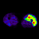
On the left, an example of blood flow image calculated using ARG method from legs.
ARG method for regional TACs
It is possible to apply ARG method to regional TACs, although this may be useful only in simulation studies to study the biases introduced by the ARG method.
For regional calculation, follow the step-by-step instructions above, except that in step 2 integrate the regional TAC data using program dftinteg, and in step 3 convert the TAC integrals to perfusion values using program taclkup.
Bias caused by vascular radioactivity
In the ARG method the contribution of vascular radioactivity is usually assumed to be negligible, which leads to overestimation of the perfusion estimates:


See also:
References:
Ginsberg MD, Howard BE, Hassel WR. Emission tomographic measurement of local cerebral blood flow in humans by an in vivo autoradiographic strategy. Ann Neurol. 1984; 15: S12-S18. doi: 10.1002/ana.410150704.
Herscovitch P, Markham J, Raichle ME. Brain blood flow measured with intravenous H215O. I. Theory and error analysis. J Nucl Med. 1983; 24: 782-789. PMID: 6604139.
Herscovitch P, Raichle ME. What is the correct value for the brain-blood partition coefficient for water? J Cereb Blood Flow Metab. 1985; 5: 65-69. doi: 10.1038/jcbfm.1985.9.
Howard BE, Ginsberg MD, Hassel WR, Lockwood AH, Freed P. On the uniqueness of cerebral blood flow measured by the in vivo autoradiographic strategy and positron emission tomography. J Cereb Blood Flow Metab. 1983; 3: 432-441. doi: 10.1038/jcbfm.1983.69.
Iida H, Kanno I, Miura S, Murakami M, Takahashi K, Uemura K. Error analysis of a quantitative cerebral blood flow measurement using H215O autoradiography and positron emission tomography, with respect to the dispersion of the input function. J Cereb Blood Flow Metab. 1986; 6: 536-545. doi: 10.1038/jcbfm.1986.99.
Liukko K. Effects of decay correction in autoradiography method. TPCMOD0037.
Raichle ME. Quantitative in vivo autoradiography with positron emission tomography. Brain Res Rev. 1979; 1: 47-68. PMID: 385113.
Raichle ME, Martin WRW, Herscovitch P, Mintun MA, Markham J. Brain blood flow measured with intravenous H215O. II. Implementation and validation. J Nucl Med. 1983; 24: 790-798. PMID: 6604140.
Ruotsalainen U, Raitakari M, Nuutila P, Oikonen V, Sipilä H, Teräs M, Knuuti J, Bloomfield PM, Iida H. Quantitative blood flow measurement of skeletal muscle using oxygen-15-water and PET. J Nucl Med. 1997; 38:314-319. PMID: 9025761.
Tags: Autoradiography, Look-up table, Perfusion, Parametric image, Phosphor imaging
Updated at: 2019-03-17
Created at: 2008-05-12
Written by: Vesa Oikonen