Long time frames in Patlak analysis
Use of Patlak plot requires calculation of integral over time (area-under-curve, AUC) of the input function starting from the tracer administration time, although the PET scan can be started later. When arterial plasma curve (PTAC) is used as input function, blood samples must be collected frequently to get a precise estimate of its AUC. If PET scan is started at the tracer administration time, and input function can be derived from the image, it is not necessary to collect short time frames - to obtain the AUC during a time frame, the radioactivity concentration can be simply multiplied by the frame length, and the AUC obtained this way is not biased at the frame end times even with long the frame lengths. This is one of the reasons that both the frame start times and end times or frame durations are stored in PET image and TAC data files.
Since the Patlak and Logan plots (and FUR) only need AUC from the early time range (before the start of the linear phase) the first image time frames can be long, even when extracting blood or reference tissue from the image. This is shown in the following simulation, using FDG as an example. The data and script are available in gitlab.utu.fi/vesoik/simulations.git.
Simulation
Mathematical function that describes the population average of FDG concentrations in arterial plasma is used to create FDG PTAC at 3 s sample intervals. Tissue curve (TTAC) is simulated using the PTAC as input function, and irreversible 2TCM, with typical parameters for the brain grey matter: K1=0.09 mL*(min*mL)-1, K1/k2=0.41 mL*mL-1, and k3=0.11 min-1. Blood volume is not considered in this simulation (VB=0). With these parameters, the net influx rate estimated using Patlak analysis should give value Ki=0.0300444 mL*(min*mL)-1, as can be calculated from equation for Ki in 2TCM:
Indeed, when the plasma and tissue data with 3 s sample intervals are used to calculate the Patlak plot, starting the linear fit at 15 min, the resulting Ki is 0.03000 mL*(min*mL)-1.
Next the PET time frames are simulated by calculating average of PTAC or TTAC during each time frame. For this example, each nine frames are set to the length of 10 min.


When these simulated 10 min frames are applied to both PTAC and TTAC, then patlak still computes correct Ki, 0.03004 mL*(min*mL)-1, because the data files contain frame start and end times, and the software can correctly account for these in AUC calculation. But if we remove this information from the TTAC and PTAC files, and save only the frame middle times, then AUC cannot be calculated correctly, and the resulting Ki is 0.03180 mL*(min*mL)-1 (overestimated, because input function AUC is underestimated). Note that when time frames are long, the image-derived blood TAC may seem like the peak was missed, and the blood vessel may be hard to detect in the image.
The simulation continues by creating a simple dynamic image from the data with the nine 10 min frames.
Simulated image is stored in ECAT format, but converted also into NIfTI format, so that it can be used in software that does not support ECAT. When Patlak plot is computed pixel-by-pixel, and the Ki is derived from the region representing the tissue, a correct value 0.03003 mL*(min*mL)-1 is retrieved.
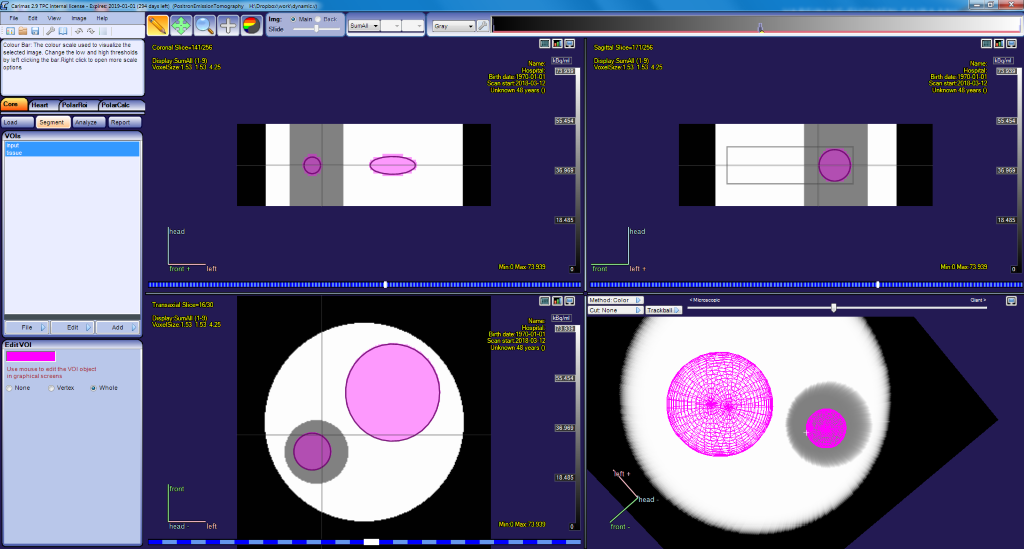
We can now load the dynamic image in Carimas, draw ROIs in the tissue and input regions, and calculate Patlak inside Carimas:

The TACs calculated from the tissue and plasma region can be saved in TAC file in Carimas, and if this file is used to compute Patlak outside Carimas, the Ki estimate is still correct, 0.03004 mL*(min*mL)-1, because the data files saved in Carimas contain the frame start and end times.
See also:
- MTGA
- Input function
- Long time frames in myocardial [15O]H2O analysis
- Time frames of image-derived input function
- Simulation of PET time frames
- Simulations in GitLab
Literature
Buchert R, van den Hoff J, Mester J. Accurate determination of metabolic rates from dynamic positron emission tomography data with very-low temporal resolution. J Comput Assist Tomogr. 2003; 27(4): 597-605. doi: 10.1097/00004728-200307000-00026.
Tags: Patlak plot, Time frame, AUC, Simulation
Updated at: 2018-05-26
Created at: 2018-03-13
Written by: Vesa Oikonen